In B2B data, company size is a foundational attribute. It drives segmentation, scoring models, and market analysis. Yet in any large company universe, some entities can't be sized through conventional means. They don't file publicly, they don't maintain a visible hiring presence, and they don't appear in the databases that traditional employee-count providers rely on.
These aren't all micro-businesses. Many are mid-market companies that operate with meaningful headcount but leave a thin digital footprint. Getting their size wrong doesn't just hurt model metrics; it degrades every downstream system that depends on accurate firmographics.
We set out to close this gap by leveraging signals already flowing through our multi-source data pipeline for better inference.
The setup: In a typical B2B company universe, the majority of entities have a known employee range from one or more data sources. A subset has insufficient signal for conventional sizing. These are the inference targets.
Why This Is a Hard Classification Problem
Ordinal Multi-Class, Not Binary
We classify into multiple ordinal tiers spanning single-digit headcount to 10,000+. Standard accuracy doesn't work here because the tiers are ordered: predicting one tier off is a small miss, while predicting the opposite end of the spectrum is a disaster. Those aren't the same kind of error.
Our primary metric is tier distance: how many buckets off was the prediction. We report adjacent accuracy (within ±1 tier) alongside exact match. For an entity with true tier y and predicted tier ŷ:
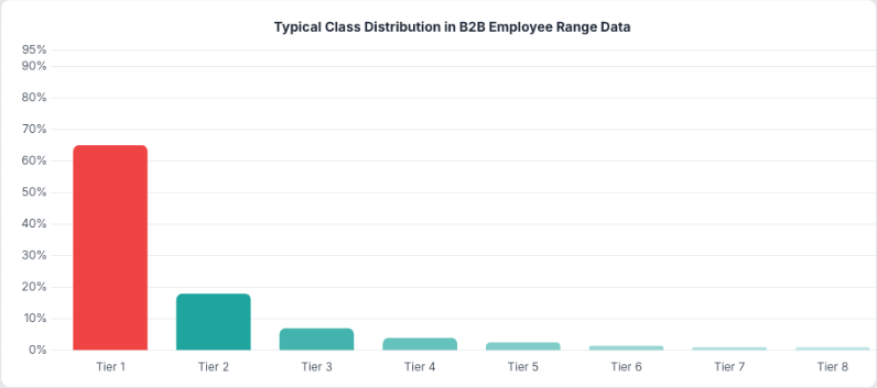
d(y, ŷ) = |τ(ŷ) − τ(y)|Extreme Class Imbalance
The population distribution follows a heavy power law. The vast majority of entities fall into the smallest tiers. A model that always predicts the dominant class would report high accuracy and be completely useless. So we train and evaluate on a stratified, balanced set where each tier gets equal representation. On that balanced set, a naive baseline is low. Our best model reaches a significant multiple of that baseline. Getting there took more than picking the right algorithm.
Covariate Shift: The Train-Inference Distribution Mismatch
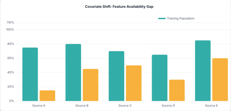
The harder problem is that the entities we want to classify don't look much like the entities we trained on. Training data naturally comes from well-documented, data-rich records that appear across many sources. Inference targets tend to have sparser signals and fewer data sources present.
Some feature groups show meaningful availability gaps between the two populations. A model that leans heavily on data-rich features will degrade in production. Train on one distribution, deploy on another, and you'll find out quickly.
Training Under Covariate Shift: Feature Group Dropout
The Technique
The fix is borrowed from deep learning: dropout. But instead of randomly zeroing individual neurons or features, we zero entire feature groups at once, at rates calibrated to match how often each data source is actually missing at inference time.
x̃(g) = x(g) · zg, zg ~ Bernoulli(1 − pg)The idea is simple: partition your feature vector by data source. For each training sample, independently decide whether to zero out each group. Set the dropout probability for each group to approximate the missingness rate you expect at inference.
| Feature Group Type | Dropout Rate | Rationale |
|---|---|---|
| Low-coverage source | High | Rarely available for inference targets |
| Medium-coverage source | Moderate | Partially available at inference |
| High-coverage source | Low | Mostly available, small gap |
| Universal source | 0% | Nearly always present |
for sample xᵢ in training set:
    for group g in feature_groups:
        sample zg ~ Bernoulli(1 − pg)
        if zg == 0:
            set x(g) ← 0
Why groups, not individual features?
In multi-source data, missingness isn't random at the feature level. It's structured at the source level. Either you have data from a particular source for an entity or you don't. You'd never see some features from a source present while others are missing. Standard per-feature dropout creates sparsity patterns that don't match what actually happens in production. Group-level dropout replicates the real failure mode.
Impact
Without dropout, accuracy on a sparse evaluation set (mimicking real inference conditions) was dramatically lower than on the held-out test drawn from the same rich distribution. Feature group dropout closed the majority of this gap:
| Evaluation Scenario | Without Dropout | With Dropout | Change |
|---|---|---|---|
| Held-out (full coverage) | High | Slightly lower | Mild regularization cost |
| Sparse (mimics real-world data) | Low | Substantially higher | Large improvement |
The held-out accuracy drops slightly (dropout acts as a regularizer), but sparse accuracy improves dramatically. This is exactly the right trade-off for a model that will operate on sparse data in production.
Model Architecture
XGBoost with Softmax Objective
We use XGBoost with a softmax objective over K classes. For each input, the model outputs a full probability distribution across all tiers, not just a single prediction. The argmax gives the predicted tier; the max probability gives the confidence score.
P(y = k | x) = exp(fk(x)) / Σⱼ exp(fⱼ(x))Having calibrated probabilities is useful: different downstream systems can decide their own precision-recall tradeoff. Use only high-confidence predictions for precision-sensitive applications; use everything when coverage matters more.
Full Pipeline
Training: Multi-Source Data → Stratified Sampling (balanced across tiers) → Feature Group Dropout (calibrated to inference sparsity) → XGBoost (multi:softprob) → Model ArtifactsInference: Company (sparse features) → Feature Engineering → XGBoost Predict → P(tier₁), …, P(tierₖ)
From the probability vector we derive:
- Predicted Tier: argmax of the probability distribution
- Confidence Score: max probability across tiers
- Binary Flags: thresholded aggregates for downstream classification
Feature Engineering: The Concepts That Mattered
We draw features from multiple orthogonal data sources, each capturing a different facet of company scale. Rather than walk through the full feature inventory, we'll focus on two engineering decisions that had outsized impact.
Identifying Enterprise-Indicative Signals
Not all signals correlate equally with company size. We identified a subset of signal categories where adoption rates differ dramatically between the smallest and largest entities — categories where large enterprises are far more likely to show presence than small businesses. Counting how many of these enterprise-indicative signals an entity exhibits produces a simple but powerful discriminator.
Let E be the set of enterprise-indicative signal categories, and Si the signals observed for company i:
N_enterprise(i) = |Sᵢ ∩ E|This count is near-zero for small companies and consistently elevated for large enterprises.
Multiplicative Gating: Suppressing Misleading Features
Web presence (a proxy for a company's online visibility and domain authority) is one of the strongest individual predictors of company size. Larger companies naturally have more pages, more backlinks, more brand searches. But the correlation breaks down in systematic ways. Small entities can inherit inflated web authority through factors unrelated to their actual size, such as generic domain names, content-heavy business models, or keyword overlap with larger brands.
These cases share one property: high web presence with zero enterprise infrastructure. A genuine large enterprise doesn't just have a well-ranked website. It runs enterprise-grade software stacks. A small firm with an inflated domain never does.
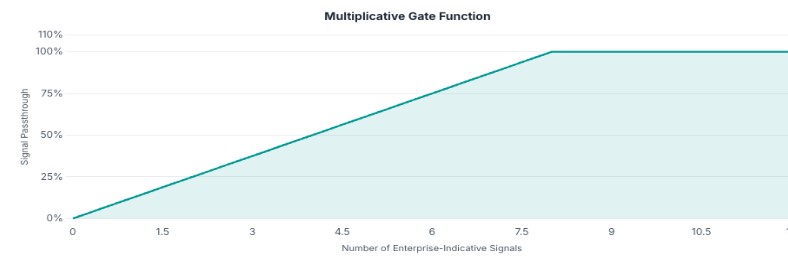
The fix is to gate the web presence signal on an independent corroborator of true company scale, the enterprise signal count described above:
GatedSignalᵢ = WebPresenceᵢ · min(N_enterprise(i) / α, 1)Gate ∈ [0, 1]
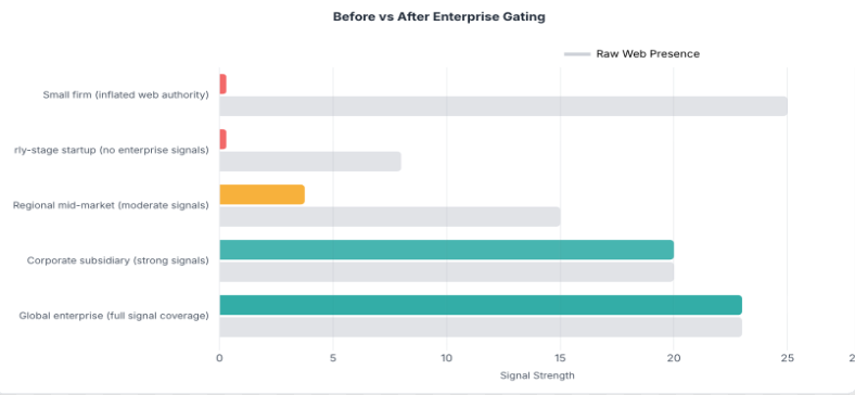
| Scenario | Web Presence | Enterprise Signals | Gate | Gated Output | Effect |
|---|---|---|---|---|---|
| Small firm with inherited high authority | High | 0 | 0.0 | 0.0 | Misleading signal fully suppressed |
| Large enterprise, legitimate authority | High | Many | 1.0 | High | Signal fully preserved |
| Mid-size company, moderate signals | Moderate | Few | 0.25 | Low-Moderate | Signal scaled proportionally |
An Illustrative Example
Consider a small professional services firm with an unusually high web presence score, perhaps due to a generic domain name or strong SEO practice. The firm has no enterprise-grade technology signals.
Before gating: High web presence. Enterprise signal count: 0. The model predicts a very large company with high confidence. Off by many tiers — a catastrophic miss.
After gating: Gated signal drops to near zero. The model falls back on the remaining features and correctly predicts a small company. Exact match.
The raw web presence score was that misleading. The gate suppressed it, and the model fell back on features that correctly indicated a small company. One multiplicative feature turned a catastrophic miss into an exact match.
The Evolution: Rules to Gradient-Boosted Trees
Phase 1: Heuristic Scoring
The first version was rule-based: a weighted sum of features with tier thresholds tuned by hand. The fundamental limitation: a linear combination can't capture conditional interactions. A particular signal means something very different for a 2-person company than for a 200-person one.
Phase 2: Gradient-Boosted Trees
Trees handle this naturally. Each split conditions on all previous splits, so the model can learn things like "high web presence only matters when the company also shows enterprise-grade signals." This kind of compound logic is simply beyond what a linear model can express.
The progression tells a clear story: moving from rules to trees was valuable, but the biggest gains came from feature engineering: adding web structure signals, fixing data quality issues, and introducing the multiplicative gating mechanism. The model architecture stayed the same throughout; what changed was what we fed it.
Pitfalls in Tree-Based Ordinal Classification
Data Quality Over Feature Quantity
In multi-source data, a common trap is chasing new features while existing ones carry systematic noise. Data sources can contain synthetic or templated entries (auto-populated URLs, default values) that apply universally regardless of entity size. When these make it into a feature, they dilute its discriminating power to near zero.
The fix is straightforward: audit feature-level signal quality before engineering new ones. Filtering a single polluted source can recover more discriminating power than adding an entirely new feature group.
A single data quality fix can outperform adding entire new feature groups.
Why Monotonic Transforms Don't Help Trees
When a feature is noisy or misleading for a subpopulation, a natural instinct is to transform it: log(log(x)), √log(x), sigmoid normalization, percentile binning. With tree-based models, all monotonic transforms produce identical splits.
This is a fundamental property of axis-aligned decision trees. A tree splits on thresholds:
1[xⱼ > t] = 1[f(xⱼ) > f(t)] ∀ monotonic fThe tree searches every possible threshold, so applying f just shifts t to f(t). Same partition, different number. No new information has been added.
To change a tree model's behavior, you must provide new information: additional features, interaction terms, or non-monotonic transformations. Monotonic transforms are mathematically a no-op.
Pre-Computed Interactions as an Alternative
When Feature A is misleading for a subpopulation that Feature B can identify, the model needs to learn a conditional: "trust A only when B is present." With many features and limited tree depth, the model may not find the right split sequence. Feature A wins a split before Feature B gets a chance to filter it.
Pre-computing the interaction (e.g., A · g(B)) solves this by encoding the conditional directly. The tree can split on the interaction feature in one step instead of learning a multi-level sequence. In practice, this type of engineering tends to disproportionately reduce catastrophic errors — the predictions that are off by many tiers — even when the overall accuracy improvement looks small.
Key Results
A Counterintuitive Result
The model is more accurate on sparse data than on rich data. That sounds wrong. Here's why it's not.
The two evaluation sets measure different things. The held-out set is balanced: equal entities per tier, including the rarest tiers where training examples are fewest. Every tier drags on the average equally. The sparse (production-like) set uses the natural distribution, where the most common tiers dominate.
Neither number is "wrong." The balanced set measures model capacity across the full range. The sparse set measures what production actually looks like. Both matter, and the gap between them reveals where the model is strong versus where it still has room to improve.
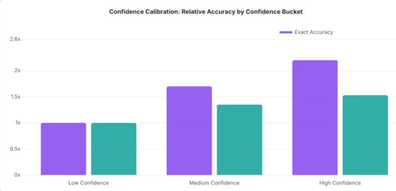
Confidence Calibration
The max softmax probability turns out to be a reliable confidence signal. High-confidence predictions are substantially more accurate than low-confidence ones. This means the model has a reasonable sense of when it's guessing. Downstream systems can set their own precision-recall tradeoff: use only high-confidence predictions for precision-sensitive applications, or accept all predictions for full coverage.
Tier Distance Distribution
The distribution of prediction errors tells a strong story:
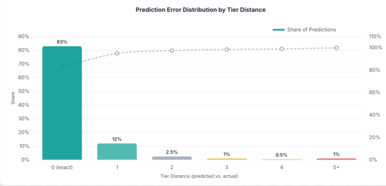
| Tier Distance | Share of Predictions |
|---|---|
| 0 (exact match) | 83% |
| 1 | 12% |
| 2 | 2.5% |
| 3 | 1% |
| 4 | 0.5% |
| 5+ | 1% |
The vast majority of predictions land within 1 tier of ground truth.
Closing Thought
The biggest accuracy gains in this project didn't come from model selection or hyperparameter tuning. They came from understanding the data deeply enough to ask the right questions. Why are small entities being misclassified at the extremes? Because a key feature is misleading without corroboration. Why does the model degrade on inference targets? Because training data is structurally different from what we see in production.
Each of those questions led to a specific, targeted fix. The model stayed the same throughout. What changed was what we fed it.
For anyone building classifiers on messy, multi-source data: spend less time on architecture search and more time on error analysis. The predictions will tell you exactly what's broken, if you look at them one at a time.
ML engineering at its core is not about models. It's about data. The model is just the mechanism that turns your understanding of the data into predictions. The deeper that understanding, the better the predictions, regardless of what's under the hood.